3 Methodology and Results
3.1 Statistical Tests
Prior to conducting any statistical tests, we checked the assumptions for normality, equal variance, and independence. Since we had a relatively small data set, we used the Shapiro-Wilk test to assess whether the shops were normally distributed and Levene’s test for equality of variances (F-test) between shops in Raleigh and NYC. While the normality assumption did not hold (p= 3.81 x 10⁻⁴), we were able to confirm the equality of variances (p= 0.81). For the independence assumption, we assumed each shop was independent; however, we created a feature called “chain” that provided a binary flag if there were multiple locations.
Thus, we performed a Wilcoxon’s 2 sample t-test on the two different groups. We found that boba shops in Raleigh were significantly different from boba shops in NYC, with a p-value of 4e-03. All statistical tests utilized a significance level (alpha) of 0.05. The mean rating of shops in Raleigh was 4.16 (variance 0.32), while the mean rating in NYC was 3.84 (variance 0.35). This resulted in a difference in means of 0.35.
With our intial hypothesis confirmed by the statistically significant difference, our focus shifted to a more detailed comparison of boba shops in Raleigh and NYC. We decided to utilize both an explanatory and predictive approach, running a linear regression model for explainability and a random forest model for predictability.
3.2 Linear Regression Model
To utilize an explanatory approach, we built two different variable selection models with rating as the target variable using forward stepwise regression. One model was for Raleigh while the other model was for New York City. After setting a full model and an empty model separately for the Raleigh and NYC data sets, we ran stepwise selection with k, the number of model parameters, set to 2. The following code chunks display the stepwise selection code.
3.2.1 Raleigh Variable Selection
##
## Call:
## lm(formula = Rating ~ Juice.Bars...Smoothies_ind + Asian.Fusion_ind +
##     Coffee...Tea_ind + Bakeries_ind + Tea.Rooms_ind, data = raleigh_df)
##
## Residuals:
##      Min       1Q   Median       3Q      Max
## -1.03755 -0.27358  0.06431  0.22642  0.72642
##
## Coefficients:
##                             Estimate Std. Error t value Pr(>|t|)
## (Intercept)                  4.27358    0.09213  46.385  < 2e-16 ***
## Juice.Bars...Smoothies_ind1 -0.73603    0.16208  -4.541 5.76e-05 ***
## Asian.Fusion_ind1           -0.97265    0.31419  -3.096  0.00373 **
## Coffee...Tea_ind1            0.39814    0.14467   2.752  0.00912 **
## Bakeries_ind1               -0.52265    0.31419  -1.663  0.10467
## Tea.Rooms_ind1               0.47642    0.31483   1.513  0.13871
## ---
## Signif. codes:  0 '***' 0.001 '**' 0.01 '*' 0.05 '.' 0.1 ' ' 1
##
## Residual standard error: 0.4257 on 37 degrees of freedom
## Multiple R-squared:  0.4623, Adjusted R-squared:  0.3896
## F-statistic: 6.361 on 5 and 37 DF,  p-value: 0.0002349
3.2.2 NYC Variable Selection
##
## Call:
## lm(formula = Rating ~ Authenticity + City + Creperies_ind + Taiwanese_ind +
##     Juice.Bars...Smoothies_ind, data = nyc_df)
##
## Residuals:
##      Min       1Q   Median       3Q      Max
## -1.02837 -0.24584  0.00181  0.27797  1.47163
##
## Coefficients:
##                             Estimate Std. Error t value Pr(>|t|)
## (Intercept)                   5.1026     0.4282  11.917  < 2e-16 ***
## Authenticity1                -0.4408     0.1286  -3.427  0.00114 **
## CityElmhurst                 -1.0037     0.4709  -2.131  0.03738 *
## CityFlushing                 -1.1334     0.4276  -2.651  0.01038 *
## CityForest Hills             -0.9790     0.5428  -1.804  0.07659 .
## CityFresh Meadows            -0.4075     0.4518  -0.902  0.37089
## CityJackson Heights          -0.1618     0.6574  -0.246  0.80647
## CityNew York                  0.1178     0.5510   0.214  0.83149
## CityQueens                   -0.7002     0.4608  -1.520  0.13411
## CityRego Park                -1.1618     0.6574  -1.767  0.08255 .
## Creperies_ind1               -1.3989     0.4500  -3.109  0.00293 **
## Taiwanese_ind1                0.4680     0.2265   2.066  0.04338 *
## Juice.Bars...Smoothies_ind1  -0.3063     0.1493  -2.052  0.04480 *
## ---
## Signif. codes:  0 '***' 0.001 '**' 0.01 '*' 0.05 '.' 0.1 ' ' 1
##
## Residual standard error: 0.4939 on 57 degrees of freedom
## Multiple R-squared:  0.4173, Adjusted R-squared:  0.2946
## F-statistic: 3.401 on 12 and 57 DF,  p-value: 0.000866
The linear regression for Raleigh that had the lowest AIC of -67.90 included three features of the juice bar/smoothie indicator, Asian fusion indicator, and coffee/tea indicator. The best linear regression for NYC had an AIC of -87.14 and found the features of authenticity, city, creperies, Taiwanese, and juice bar/smoothie indicator. Among the two sites, there were seven distinct features observed between the two variable selection models. The only shared feature was the juice bar/smoothie indicator, leading us to wonder if the random forest features would be similar.
3.3 Random Forest Model
While random forest models are generally used for prediction, we used their ability to assess variable importance as a comparison point for the linear regression model. Our feature ranking was determined by the percent increase in the mean squared error (MSE). We assessed the variable importance of our predictive model output with a variable called “random”, seen in the plots below.
The Raleigh plot of variable importance is displayed below:
## randomForest 4.7-1.1## Type rfNews() to see new features/changes/bug fixes.##
## Attaching package: 'randomForest'## The following object is masked from 'package:dplyr':
##
## combine## The following object is masked from 'package:ggplot2':
##
## margin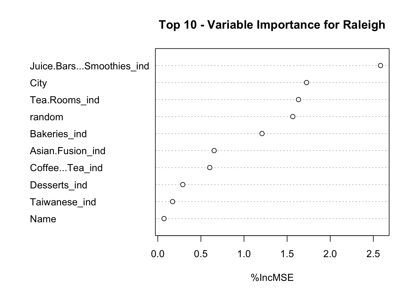
The top ten important variables for the predictive model in Raleigh were similar to the linear regression model. Of the three explanatory variables of the linear regression (juice bar/smoothie indicator, Asian fusion indicator, coffee/tea indicator), only juice bar/smoothie appeared before the random variable. A high overlap between explanatory and predictor variables allows us to infer that there are similar attributes that go into forming and retaining a good Raleigh boba shop. These include:
Having a variety of options, such as smoothies and juices.
Appealing to the “fusion” audience rather than as an authentic boba shop.
Being tagged as a tea room.
Having food options, such as baked goods.
Offering coffee choices.
The NYC plot of variable importance is displayed below:
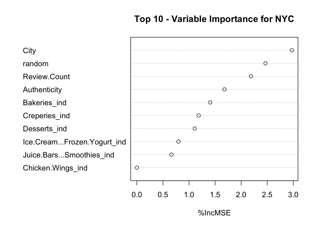
The top importance variables output from the random forest for New York City seemed to focus on location, seen in the ranking of the “city” feature.
It’s important to note that the “city” variable was important in both the Raleigh and NYC variable importance outputs from our random forests; this may indicate that the shop’s location is a large factor in a Yelp rating. This output prompted us to visualize our dataset and explore the map of boba shops across both data sets.
3.4 Visualization
We utilized the visualization platform Tableau to display both Raleigh and NYC boba shops by longitude and latitude. The feature “city” in the data set indicated that Raleigh’s n = 43 boba shops spanned 9 towns, while NYC’s n = 70 boba shops spanned 10 neighborhoods. We noticed that shops in NYC tended to be more concentrated or in closer proximity to each other than shops in Raleigh. This indicates that there was more competition in close proximity in NYC than in Raleigh. This visualization reiterated the results from both the variable selection model and the predictive random forest model, specifically with the random forest model confirming that the “city” feature was important in mean boba shop rating outcomes. We hypothesize this could be attributed in part to physical shop proximity.
The Tableau visualization, found in the Github repository, reinforced the findings obtained from both the linear regression model and the predictive random forest model. Combined, they highlighted the most impactful features, indicating a distinct underlying difference in features contributing to boba shop ratings on Yelp.